Description

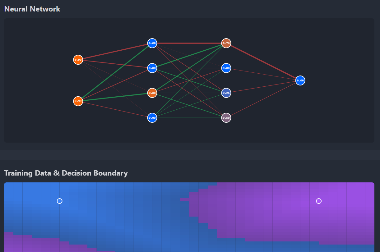
This project is an interactive visualization of a neural network learning in real-time. Watch activations flow forward (blue particles) and gradients flow backward (red particles) during training, while the network learns to classify 2D datasets.

The visualization demonstrates fundamental concepts in deep learning:

• Forward propagation - Input signals flow through the network layer by layer
• Backpropagation - Gradients flow backward to update weights
• Decision boundaries - Visual representation of what the network has learned
• Loss curves - Track learning progress over time

The demo features:

• Network architecture controls - Adjust hidden layer sizes dynamically
• Multiple datasets - XOR (non-linearly separable), Circle, Spiral, and Diagonal problems
• Activation functions - Switch between Sigmoid, ReLU, and Tanh
• Live animations - See blue particles flow forward and red particles flow backward
• Decision boundary visualization - Color-coded regions show network predictions
• Performance metrics - Track loss, accuracy, and training progress
• Interactive training - Play, pause, step through, or reset training

The network is implemented from scratch in JavaScript (no ML libraries like TensorFlow for the core logic), demonstrating the mathematics behind neural networks. The visualization shows:

• Node colors indicating activation magnitude (blue = low, red = high)
• Edge thickness showing weight magnitude
• Edge colors showing weight sign (green = positive, red = negative)
• Animated particles representing data and gradient flow

Live Demo

The live demo is available to try out. You can:

• Adjust the network architecture (2 → 4 → 4 → 1 or customize hidden layers)
• Switch between different activation functions to see how they affect learning
• Control the learning rate and training speed
• Select different datasets to test the network’s ability to learn various patterns
• Watch the network struggle with simple problems and succeed with proper architecture
• Step through training one epoch at a time to understand the learning process
• See the decision boundary evolve as the network learns

The demo clearly shows why XOR cannot be solved with a single-layer perceptron but is easily solved with hidden layers, demonstrating the power of deep learning for non-linear problems.

Technical Implementation

Core Components

Neural Network Engine (NeuralNetwork.js):

• Forward propagation with matrix operations
• Backpropagation with gradient computation
• Xavier weight initialization
• Multiple activation functions (sigmoid, ReLU, tanh)
• MSE loss calculation

Animation System (animations.js):

• Particle-based visualization of data flow
• Forward pass: blue particles from input to output
• Backward pass: red particles from output to input
• Easing functions for smooth motion
• Staggered timing for layer-by-layer effect

Training Datasets (datasets.js):

• XOR: Classic non-linearly separable problem (4 points)
• Circle: Inner circle vs outer ring classification (50 points)
• Spiral: Two interleaved spirals (100 points)
• Diagonal: Simple linearly separable problem (50 points)

Visualization:

• Canvas 2D for network graph and decision boundary
• Chart.js for real-time loss plotting
• Color-coded nodes showing activation values
• Weighted edges showing connection strength
• Grid-based decision boundary with confidence coloring

Key Concepts Demonstrated

Backpropagation

The visualization makes backpropagation tangible by showing red particles flowing backward through the network. The chain rule of calculus is animated as gradients propagate from the output layer back to the input layer.

Decision Boundaries

The decision boundary grid shows what the network has learned. As training progresses, you can watch the boundary shift and curve to separate the classes. The color intensity shows prediction confidence.

Activation Functions

Switching between sigmoid, ReLU, and tanh shows how activation functions affect learning speed and convergence. ReLU often converges faster but can suffer from dying neurons. Sigmoid works well for binary classification but can have vanishing gradients.

Learning Rate

The learning rate slider demonstrates the bias-variance tradeoff. Too high and the network oscillates or diverges. Too low and learning is painfully slow. Finding the sweet spot is key to successful training.

Experiments to Try

• Architecture matters: Try solving XOR with [2, 2, 1] vs [2, 8, 8, 1]. Does bigger always mean better?
• Learning rate tuning: Set learning rate to 0.01 vs 1.0 on the spiral dataset. What happens?
• Activation functions: Compare sigmoid vs ReLU on the circle dataset. Which converges faster?
• Dataset difficulty: Train on diagonal (easy) then switch to spiral (hard) without resetting. Does transfer learning help?
• Overtraining: Let the network train for 500+ epochs. Does accuracy keep improving?

Future Enhancements

Potential improvements for the demo:

• Momentum and Adam optimizer - Show how modern optimizers converge faster
• Batch normalization - Visualize how it stabilizes training
• Dropout visualization - Show neurons being randomly disabled
• Regularization effects - L1/L2 penalty visualization
• Mini-batch training - Animate batch-wise updates
• 3D visualization - For datasets with 3 input features
• Export trained models - Save weights and reload later

References

• Backpropagation - Wikipedia
• Universal Approximation Theorem - Why neural networks work
• Activation Functions - Comparison of different functions
• Gradient Descent - Optimization algorithm
• Neural Networks and Deep Learning - Michael Nielsen’s free book
• 3Blue1Brown Neural Networks Series - Visual explanations